
Dynamic transshipment policies for interstate moving companies with load uncertainty
Interstate moving companies move household items from one location to another. They often optimize their routes by assigning a truck to \(n > 1\) households in a single day within a region, move the items to a storage location and then solve a dispatch problem to deliver each household’s items from storage to the new location within a time window. A crucial step in planning is knowing in advance the size of the cargo that will have to be picked up. This was traditionally done through an examination by an agent before the scheduled move. With recent changes due to COVID restrictions, moving companies rely on customer’s estimate of volume and size of their items. These estimates often have errors and may cause order cancellations at the last minute, either due to price difference from the initial quote or limited capacity of the assigned truck. As a result, an additional source of uncertainty is introduced in the planning of the moving company. We propose a stochastic optimization framework that incorporates this uncertainty in scheduling load shipments between moving companies regional warehouses.
 |
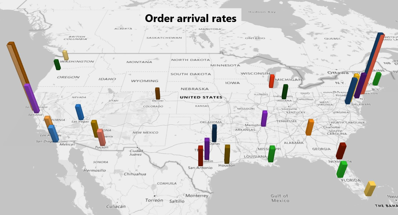 |
| Fig. 1: Problem Overview | Fig. 2: Order arrival rates |
Fig 1 above shows an overview of the problem where orders from different region arrive into the origin warehouse. This process is not modeled via our solution as we assume that once an order arrives, its pickup and transfer to origin warehouse are deterministically determined. Then, the order is shipped from the origin warehouse to a destination warehouse. In this process, the destination warehouse is predetermined. However, the order can be immediately shipped to the destination warehouse or it can be delayed to match with another order (to the same destination) given the remaining truck capacity. Transferring from destination warehouse to destination is also assumed to be deterministically determined and thus is not considered in our formulation.
Fig 2 shows the order arrival process. Note that, to ease computation, the order arrival process of only a certain set of cities are considered in the following example.
1- Dynamic Programming Model
Once an order is received by the moving company, its origin, destination, pickup time, and estimated size are known. In the following model, the actual pickup time and final delivery are assumed to be deterministic and therefore of no consequence to the model. However, the time an item is kept in the moving company’s regional warehouse before shipping to the destination warehouse is stochastic. This time is captured in the following model where the value function is incentivized to minimize it by assigning a penalty to delayed time after pickup.
Decision time:
A decision on whether to ship the order immediately or delay it to bundle with the next shipments is made every time a pickup time arrives.
State space:
\[S:=\bigg\{s=\big(\text{order},\,\text{status}\big)=\big(w^o_i, w^d_i, t^p_i, s_i, f_i\big),\,\, i= 1, 2, \ldots\bigg\},\]where \(w^o_i,\,w^d_i\in\mathbb{W}:=\{1, 2, \ldots, \|W\|\}\) denote the origin and destination of the \(i^\text{th}\) order, \(t^p_i\) is the pickup time, and \(s_i\) is the size of the order. Shipment status of order \(i\) is denoted by the binary variable \(f_i\) where \(1\) indicates that the order is shipped while \(0\) shows delay of shipment.
Error adjustment: It is assumed that \(s_i\) may be estimated with error by the customer and its true size is only revealed at the time of pickup. The estimate error may be normal, or skewed to right and left to capture overestimation and underestimation.
Action space:
\[X:=\bigg\{x^t_i\in\{0, 1\},\,\, i= 1, 2, \ldots; N^t_{o, d}\in\mathbb{Z}_{+},\,\, o, d\in\mathbb{W}\bigg\},\]where \(x^t_i\) is a binary variable which is \(1\) if order \(i\) is shipped at time \(t\), and \(N^t_{o,d}\) is the number of trucks required to ship orders from origin \(o\) to destination \(d\).
1- Note that orders cannot be shipped if their pickup time has not arrived yet:
\[t^p_i x^t_i \leq t, \qquad \forall i = 1, 2, \ldots.\]2- Also, to determine the minimum number of trucks needed to ship all orders from origin \(o\) and destination \(d\):
\[\begin{align*} & \min N^t_{o, d} &\\ \text{subject to} & \sum_i u_{ij} \leq \nu y_j, & \forall j = 1, 2, \ldots, n,\\ & \sum_j y_j \leq N^t_{o, d}, &\\ & \sum_{ij} u_{ij} = n, & \end{align*}\]where \(n\) denotes the number of orders to be shipped from origin \(o\) to destination \(d\). Binary decision variable \(u_{ij}\) is \(1\) when order \(i\) is assigned to truck \(j\), and \(y_j\) is a helper binary decision variable which is \(1\) if truck \(j\) is assigned a shipment. The maximum number of truck is assumed to be equal to the number of orders. \(\nu\) represents truck capacity which, for the sake of simplicity, is assumed to be equal for all trucks.
Transition function:
\[S_{t+1} = \eta(S_t, X_t, \omega),\]where \(\eta\) is a representation of the transition function where \(\omega\) is the random element governing the arrival of new orders. Apart from the random element, state transition is straightforward as orders whose \(f_i = 1\) (i.e., orders which are already shipped) are removed from the state space.
Immediate reward:
1- Shipping revenue: Taking orders of different sizes from an origin to a destination at time \(t\) generates revenue of
\[\sum_{i}\sum_{w^o_i, w^d_i\in\mathbb{W}} P^t_{o, d} s_i x^t_i,\]where \(P^t_{o, d}\) is the price of transferring one unit of load from \(o\) to \(d\) at time \(t\).
2- Truck rent cost: Shipments from an origin to a destination are loaded onto a rented truck the cost of which is
\[\sum_{w^o_i, w^d_i\in\mathbb{W}} N^t_{o, d} C^t_{o, d},\]where \(C^t_{o, d}\) is the cost of renting a truck for shipping from \(o\) to \(d\) at time \(t\).
3- Shipment delay cost: Delaying a shipment after its pick up time results in a cost captured by
\[\sum_{i}\sum_{w^o_i, w^d_i\in\mathbb{W}} C(t - t^p_i) x^t_i,\]where \(C\) is the cost of delaying a shipment per unit of time.
The total cost of transition form state \(S_t\) to state \(S_{t+1}\) taking action \(X_t\) will be calculated by
\[h(S_t, X_t, S_{t+1}) = \sum_{i}\sum_{w^o_i, w^d_i\in\mathbb{W}} P^t_{o, d} s_i x^t_i - \sum_{w^o_i, w^d_i\in\mathbb{W}} N^t_{o, d} C^t_{o, d} - \sum_{i}\sum_{w^o_i, w^d_i\in\mathbb{W}} C(t - t^p_i) x^t_i\]Policy value function & Bellman’s equation
Implementing a policy \(\pi\) will result in the total discounted cost of
\[\mathscr{L}_{\pi}(s) = \mathbb{E}_\pi\bigg\{\sum_{t=0}^{\infty} \gamma^t\, h(S_t, X_t, S_{t+1})\,\bigg|\,S_0 = s\bigg\},\]where the optimal policy is given by
\[\sup_{\pi\in\Pi} \mathscr{L}_\pi(s)\]which is also optimal to the Bellman’s equation
\[V(s) = \min_{x_t} \mathbb{E}_x \Big[h(S_t, X_t, S_{t+1}) + \gamma^{t+1} V(S_{t+1})\, \Big|\, S_t = s\Big]\]where \(\pi(s) = (X_t)_{t=0}^\infty\).
2- Model Implementation
The following code is an attempt at implementing the dynamic programming model.
2.1- Input data
Interarrival times between order arrivals are modeled to be generated according to an exponential process with regional arrival rates (refer to Fig. 1). This is a convenient assumption because the earliest arrival will be distributed according to another exponential distribution whose mean is the sum of all regional arrival rates. However, to ease implementation, we assume an overall exponential distribution where orders arrive every three hours.
When an order arrives into the system, its origin, destination, pickup time and size must be generated. This is done with the process described below.
Origin, destination, pickup time data
A new order should arrive from a known origin for a given destination with a pickup time and an estimated size. Each order arrives according to a Poisson process and the time between pickup times are following an exponential distribution. These are standard assumptions for arrival processes and inter-event times. However, parameters of these distributions are specified arbitrarily.
Order size data
Size of each order is generated from a disjunctive set of uniform distributions designed to mimick the information in Census on the size of US households (here) and a moving company’s (AtoB estimates of the moving volume per number of rooms (here).
Error in size of data
Recall that an important component of customer estimate of size was the estimation error. However, note that the upon order arrival only the estimate size of the order is available. The true size is adjusted once the order pickup time arrives. This is done by defining <size_error_adjustment> function which is described later.
import os
import sys
import itertools
from collections import namedtuple
import numpy as np
from memoization import cached
import seaborn as sns
import matplotlib.pyplot as plt
import inspect
import pandas as pd

## data
## arbitrary: inter-pickup times are generated according to an exponential process
## where mean is the inverse of distance between location
curr_dir = os.path.dirname(os.path.abspath(inspect.getfile(inspect.currentframe())))
parent_dir = os.path.dirname(curr_dir)
dist_df = pd.read_csv(os.path.join(parent_dir, 'Data/city_dist.csv'), index_col = 0)
dist_df.replace(0, np.nan, inplace = True)

## TEMPORARY
## reduce data for now to speed up computation
dist_df = dist_df.iloc[0:3, 0:3]
min_dist = dist_df[dist_df > 0].min(axis = 0).min()
max_dist = dist_df[dist_df > 0].max(axis = 0).max()
normalized_dist_df = (dist_df - min_dist) / (max_dist - min_dist)
global pickup_attr_df
pickup_attr_df = pd.DataFrame(columns = ['org', 'dest', 'lambda', 'dist'])
for i in range(0, len(dist_df.columns)):
    for j in range(i + 1, len(dist_df.columns)):
        org = dist_df.columns[j]
        dest = dist_df.index[i]
        row  = pd.Series([org, dest, normalized_dist_df.iloc[i, j], dist_df.iloc[i, j]], index = pickup_attr_df.columns)
        pickup_attr_df = pickup_attr_df.append(row, ignore_index = True)

global truck_capacity
truck_capacity = 90
def dist_org_dest(org, dest):
    return pickup_attr_df.loc[(pickup_attr_df.org == org) & (pickup_attr_df.dest == dest), 'dist'].values[0]
2.2- State space
The state space is meant to store all the required information necessary for making decisions. According to the dynamic programming model described in Section 2, the state variable for this problem stores, order status, origin, destination, pickup time, and estimated order size. In this implementation, <generate_new_orders_func> function generates a new unassigned order (i.e., status = 0) by evaluating the minimum inter-pickup time and identify its associated origin and destination utilizing function <generate_order_pickup_func> and determining its size using <generate_order_size_func> function.
def generate_order_size_func(random_state):
    '''
        generate order size according to distribution of volumes
    '''
    volume_percent_df = pd.DataFrame([[2, 5, 0.02, 0.02],
                                      [7, 8, 0.14, 0.16],
                                      [11, 17, 0.31, 0.47],
                                      [19, 25, 0.38, 0.85],
                                      [30, 90, 0.15, 1]],
                                     columns = ['lb', 'ub', 'percent', 'cdf'])
    rand_var = random_state.uniform(low = 0, high = 1)
    intervals = volume_percent_df.cdf
    cdf_idx = np.searchsorted(intervals, rand_var, side = 'left')
    size = random_state.uniform(low = volume_percent_df.loc[cdf_idx, 'lb'],
                                high = volume_percent_df.loc[cdf_idx, 'ub'])
    return size
def generate_order_pickup_func(random_state):
    '''
        generate order origin, destination, inter pickup time
    '''
    pickup_times = random_state.exponential(scale = pickup_attr_df['lambda'])
    earliest_time = np.argmin(pickup_times)
    org = pickup_attr_df.iloc[earliest_time]['org']
    dest = pickup_attr_df.iloc[earliest_time]['dest']
    inter_pickup_time = pickup_times[earliest_time]

    return org, dest, inter_pickup_time
def generate_new_orders_func(t, random_state):
    '''
        generate a new order
        input: current time
        output: new order
    '''
    status = 0
    size = generate_order_size_func(random_state)
    origin, destination, inter_pickup_time = generate_order_pickup_func(random_state)
    s = pd.Series([origin, destination, t + inter_pickup_time, size, status],
                  index = ['org', 'dest', 'pickup_time', 'size', 'status'])
    return s
Future event list
In discrete event simulations, a future event list (fel) is maintained throughout the simulation which determines the sequence of events. Here, the fel maintains order arrival times and generates a new time as soon as an arrival time from the list is consumed. In the simulation, once the simulation clock passes an arrival time in the fel, a new order is generated and is added to the state space.
def fel_maintainer_func(current_time, random_state):
    '''
        control future event list by maintaining order arrival times
        input: current time
        output: future event list
    '''
    ## generate order arrival time from an exponential distribution
    global fel
    new_random_order_arrival_time = t + random_state.exponential(scale = 3, size = 1)[0]
    fel.append(new_random_order_arrival_time)
    fel = sorted([t for t in fel if t > current_time])
2.3- Action space
The <determine_actions_func> function creates an initial set of actions that are then filtered by the model constraints to produce a feasible decision set. Then, <minimize_num_trucks> function is used to determine the minimum number of trucks required to carry out each feasible action by solving an integer optimization described in Section 2.
def minimize_num_trucks(size_lst):
    '''
        create and solve an IP to minimize the number of trucks
        input: list of sizes to be shipped from an origin to a destination
        output: minimum number of trucks required
        model:
                        Min N
            subject to:
                        sum_i  x_ij <= capacity * y_j,      for all j in range(len(size_lst))
                        sum_j  y_j  <= N,
                        sum_ij x_ij = len(size_lst),
                        x_ij in {0, 1},
                        y_j  in {0, 1},
                        N    in {positive integers}
    '''
    from pulp import LpMinimize, LpProblem, LpStatus, lpSum, LpVariable
    model = LpProblem(name = "min-num-trucks", sense = LpMinimize)

    ## variables
    ### u_ij = 1 if size i is loaded onto truck j
    u_ij = [[LpVariable("u_{}_{}".format(i + 1, j + 1), cat = 'Binary') for i in range(len(size_lst))]
            for j in range(len(size_lst))]

    ### y_j = 1 if truck j is being used for shipping
    y_j = [LpVariable("y_{}".format(j + 1), cat = 'Binary') for j in range(len(size_lst))]

    ### N is the number of trucks needed to ship all orders
    N = LpVariable("N", cat = 'Integer', lowBound = 0)

    ## objective
    model += N

    ## constraints
    ### sum_i u_ij <= capacity * y_j; for all j
    for j in range(len(size_lst)):
        model += sum(u for u in u_ij[j]) <= truck_capacity * y_j[j]

    ### sum_j y_j <= N
    model += sum(y for y in y_j) <= N

    ### sum_ij u_ij = len(size_lst)
    model += sum(u for u_j in u_ij for u in u_j) == len(size_lst)

    ##solve model
    status = model.solve()
    if LpStatus[status] == 'Optimal':
        return model.objective.value()
    else:
        print(LpStatus[status])
        assert False, "Problem to solve for minimum number of trucks was not optimal"
def determine_actions_func(state_lst, t):
    '''
        given the state space and current time, determines all possible actions
        and number of trucks required.
        input: state space, current time
        output: action space
        process:
            1- initialize 0/1 actions for all remaining shipments
            2- remove actions that violate the time constraint
            3- determine the minimum number of trucks to ship all orders from o to d
    '''
    ## state_lst structure
    ### [origin, destination, pickup_time, size, status]

    ## initialize a set of action
    ### 1 if order i is loaded onto a truck, 0 otherwise
    remaining_states = state_lst.loc[state_lst.status == 0, ]
    num_remain_loads = len(remaining_states)
    action_lst = list(itertools.product([0, 1], repeat = num_remain_loads))

    ## constraints
    ### no order can be loaded if pickup_time > t
    def validate_pickup_time_func(action, t):
        flag = True
        for i, order_action in enumerate(action):
            if order_action == 1:
                pickup_time = remaining_states.pickup_time.iloc[i]
                if pickup_time > t:
                    flag = False
                    break
        return flag
    action_lst = [action for action in action_lst if validate_pickup_time_func(action, t)]

    ## determine number of trucks needed
    ### this is done by minimizing the number of trucks for each (org, dest) pair
    def determine_num_trucks_func(action):
        action_idx = [i for i, order_action in enumerate(action) if order_action == 1]
        action_states = remaining_states.iloc[action_idx]
        truck_dict = dict(action_states.groupby(['org', 'dest'])['size'].apply(list))
        for (org, dest) in truck_dict:
            min_num_trucks = minimize_num_trucks(truck_dict[(org, dest)])
            truck_dict[(org, dest)] = min_num_trucks

        return truck_dict
    truck_lst = [determine_num_trucks_func(action) for action in action_lst]

    return action_lst, truck_lst
2.4- Transition function
Given a state and an action, the system transitions to a new state. For example, if an order is shipped, its status changes from 0 to 1. Decision epochs are pickup times, however, between each decision, one or a few new orders may arrive for which the pickup time may be sooner or later than the pickup times for orders that are already in the list.
NOTE that the <one_step_flag> is used to distinguish between one-step look-ahead policy’s estimate of the next state, and a transition which is triggered by taking an action. This is done to distinguish between different sequences of random number. For one-step look-ahead decision making, the function uses the same sequence of random number for each state.
NOTE that in each transition the future event list is checked to see whether new orders arrive before the next pick up time. If no future order arrival are in the future event list, a new arrival is generated.
def transition_func(state_lst, action, t, random_state, one_step_flag):
    '''
        determines the new state space bases on current state space, given action, and current time
        input: current state space, action, current time
        output: next state space, next decision epoch
        process:
            1- change the status of orders that have been shipped according to action
            2- remove those orders from the state space
            3- check future event list for earliest prickup time
                3.1- if a new order arrives sooner than the earliest pickup time; generate a new order
                3.2- otherwise, generate new order arrivals
            4- move the time to next decision epoch

    '''
    global fel
    ## state_lst structure
    ### [origin, destination, pickup_time, size, status]

    ## action structure
    ### (shipped=1, not-shipped=0, ...) of the state lenght

    ## change status of orders according to shipping action
    remaining_states = state_lst.loc[state_lst.status == 0, ].reset_index(drop = True)
    for i in range(len(remaining_states)):
        if action[i] == 1:
            remaining_states.loc[i, 'status'] = 1
    assigned_states = remaining_states.loc[remaining_states.status == 1, ].reset_index(drop = True)

    ## remove already shipped order from state
    new_state_lst = remaining_states.loc[remaining_states.status == 0, ].reset_index(drop = True)

    ## determine next decision epoch; min future pickup_times
    future_pickup_time_lst = new_state_lst.pickup_time[new_state_lst.pickup_time > t]

    if len(future_pickup_time_lst) > 0:
        earliest_pickup = min(future_pickup_time_lst)
        ## check fel to determine if new orders should be generated
        earliest_order_arrivals = [time for time in fel if time > t and time <= earliest_pickup]
        if len(earliest_order_arrivals) > 0:
            for i in range(len(earliest_order_arrivals)):
                new_state = generate_new_orders_func(earliest_order_arrivals[i], random_state)
                new_state_lst = new_state_lst.append(new_state, ignore_index = True)
    else:
    ## new orders should be generated
        ## check if fel already has order arrivals
        if len(fel) > 0:
            next_order_arrival = min(fel)
            if not one_step_flag:
                fel.remove(min(fel))
            new_state = generate_new_orders_func(next_order_arrival, random_state)
            new_state_lst = new_state_lst.append(new_state, ignore_index = True)
        else:
        ## generate new order arrivals
            fel_maintainer_func(t, random_state)
            next_order_arrival = min(fel)
            fel.remove(min(fel))
            new_state = generate_new_orders_func(next_order_arrival, random_state)
            new_state_lst = new_state_lst.append(new_state, ignore_index = True)

    ## see if next decision epoch has changed
    future_pickup_time_lst = new_state_lst.pickup_time[new_state_lst.pickup_time > t]
    earliest_pickup = min(future_pickup_time_lst)

    state_lst = pd.concat([assigned_states, new_state_lst], ignore_index = True)

    return state_lst, earliest_pickup
2.5- Immediate cost/reward function
Here, the three different component of the cost/reward structure is built: Shipping revenue <shipping_revenue_func>, Truck rent <renting_cost_func>, and Shipment delay cost <delay_cost_func>. Some of the parameters used in evaluating these components are chosen arbitrarily.
def immediate_rewards_func(state_lst, action, truck_dict, t):
    '''
        immediate cost/reward structure is constructed of three components
            1 - revenue of taking load of size s from origin o to destination d
            2 - cost of renting a truck for shipment from origin o to destination d
            3 - cost of delaying order i from pickup time t
        input: current state space, action, trucks required to carry out the action, current time
        output: total immediate reward
    '''
    remaining_states = state_lst.loc[state_lst.status == 0, ]

    def shipping_revenue_func(state_lst, action):
        revenue = 0
        for i in range(len(state_lst)):
            if action[i] == 1:
                org, dest = state_lst.org.iloc[i], state_lst.dest.iloc[i]
                revenue += state_lst['size'].iloc[i] * dist_org_dest(org, dest) * 0.5
        return revenue
    immed_shipping_revenue = shipping_revenue_func(remaining_states, action)

    def renting_cost_func(truck_dict):
        cost = 0
        for (org, dest) in truck_dict:
            cost += truck_dict[(org, dest)] * dist_org_dest(org, dest) * 2
        return cost
    immed_rent_cost = renting_cost_func(truck_dict)

    def delay_cost_func(state_lst, action, t):
        cost = 0
        for i in range(len(state_lst)):
            if action[i] == 1:
                cost += (t - state_lst.pickup_time.iloc[i]) * 400
        return cost
    immed_delay_cost = delay_cost_func(remaining_states, action, t)

    return immed_shipping_revenue - immed_rent_cost - immed_delay_cost
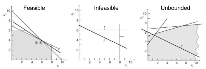
3- Overview of solution method:
The state space is continuouse and unbounded and therefore, no tractible exact solution method exist to solve the formulation above. However, approximate dynamic programming methods can identify near-optimal policies that perform reasonably well. To assess the quality of solution, the approximate dynamic policy is compared in terms of total realized revenue with a benchmark policy that immediately ships every order. The approximate dynamic programming method developed in this settings is a special case of the heuristic family of rolling-horizon policies.
3.1- Rolling-horizon policy
In this heuristic framework, it is assumed that the horizon is at decision epoch \(t+\tau\). State evolution is simulated for all possible actions and transitions until the horizon is reached. Since no further transition will happen at the horizon, its value can be derived only in terms of immediate cost/rewards. Moving backward, the best value of each previous state (w.r.t. actions) can also derived and thus the best policy is known throughout period \([t, t+\tau]\). Then, the horizon is rolled over one decision epoch and the process repeats.
The One-step look-ahead policy is a specific case of the rolling-horizon heuristic family where \(\tau = 1\). For complex stochastic problem where simulating state evolution several steps into the future is time consuming, one-step look-ahead policies proivde an easy-to-compute approximate solution method. The rolling-horizin policies are shown to be asymptotically optimal.
The function <one_step_look_ahead_policy_func> below, implements the one-step look-ahead policy by assuming that the next decision epoch is the last and thus all the remaining orders haver to be shipped immediately. Therefore, all cost/rewards are immediate and can be evaluated easily by <immediate_rewards_func> function. Enumerating over all action possible in a one-step transition will allow the function to identify the best one-step action.
NOTE that, currently, two versions of the one-step look-ahead policy are maintained: sequential and parallel. Since, one-step transitions are independent of one another, those one-step simulations can be done in parallel.
def one_step_look_ahead_policy_func(state_lst, t, random_state, seed):
    '''
        implements the one-step look-ahead policy by assuming that the next step is the end of horizon
            where all orders must be shipped
        input: current state space, current time
        output: best action, best one-step look-ahead value
        process: evaluate the immediate and one-step rewards for all possible action and choose the best
    '''
    ## parallel design
    from joblib import Parallel, delayed
    action_lst, truck_lst = determine_actions_func(state_lst, t)
    def sim_one_step(state_lst, action, truck_dict, t, random_state):
        random_state.seed(seed)
        immed_rewards = immediate_rewards_func(state_lst, action, truck_dict, t)
        new_state_lst, new_t = transition_func(state_lst, action, t, random_state, one_step_flag = True)
        new_action_lst, new_truck_lst = determine_actions_func(new_state_lst, new_t)

        ## since one-step ahead assumed to be the last step,
        ## every load would have to be shipped
        one_step_action_idx = np.argmax([sum(action) for action in new_action_lst])
        one_step_action = new_action_lst[one_step_action_idx]
        one_step_truck = new_truck_lst[one_step_action_idx]
        one_step_rewards = immediate_rewards_func(new_state_lst, one_step_action, one_step_truck, new_t)

        return immed_rewards + one_step_rewards
    total_rewards = Parallel(n_jobs = 6)(delayed(sim_one_step)(state_lst, action_lst[i], truck_lst[i], t, random_state)
                                         for i in range(len(action_lst)))

    ## sequential design
    '''
    action_lst, truck_lst = determine_actions_func(state_lst, t)
    total_rewards = []
    for i, action in enumerate(action_lst):
        random_state.seed(seed)
        immed_rewards = immediate_rewards_func(state_lst, action, truck_lst[i], t)
        new_state_lst, new_t = transition_func(state_lst, action, t, random_state, one_step_flag = True)
        new_action_lst, new_truck_lst = determine_actions_func(new_state_lst, new_t)

        ## since one-step ahead assumed to be the last step,
        ## every load would have to be shipped
        one_step_action_idx = np.argmax([sum(action) for action in new_action_lst])
        one_step_action = new_action_lst[one_step_action_idx]
        one_step_truck = new_truck_lst[one_step_action_idx]
        one_step_rewards = immediate_rewards_func(new_state_lst, one_step_action, one_step_truck, new_t)

        total_rewards.append(immed_rewards + one_step_rewards)
    '''
    ##extracting best one-step action
    best_one_step_action_idx = np.argmax(total_rewards)
    best_one_step_action = action_lst[best_one_step_action_idx]
    best_one_step_trucks = truck_lst[best_one_step_action_idx]
    best_one_step_value = total_rewards[best_one_step_action_idx]

    return best_one_step_action, best_one_step_trucks, best_one_step_value
3.2- Simulation
Starting from time t = 0, a new order arrival time is generated. Then, the pickup time of the order is generated. The algorithm checks whether any other orders will arrive between the first order arrival and the first order pick up. If not, the time moves forward to the earliest pickup time. If new orders arrive between the first arrival and the first pickup, for each new arrival, a new pickup time is generated and the time moves forward to the earliest pickup time.
3.2.1- One-step look-ahead policy
Since the sequence of random events depend on the sequence of random number, to remove the effect of psuedo-random-sequence bias, the simulation is replicated for 30 iteration and the results are averaged over the sample. In the simulation, two sequences of random numbers are maintained. The first one, overall_see, is used to control the sequence of realized events. The second one, onestep_seed, is used to control the one-step look-ahead sequence of events which will be kept the same at each decision epoch so that the one-step decision are compared with respect to the same one-step ahead simulated event.
NOTE that in the case of one-step look-ahead policy, a decision is made by simulating the system one-step forward where all the remaining shipments have to be shipped immediately.
overall_seed = 1231231
realized_value_lst = []
#policy_lst = [] #optional to uncomment
state_progression_lst = [] #optional to uncomment
trucks_lst = []
for i in range(0, 30):

    ## simulation initialization
    rand_state_onestep = np.random.RandomState()
    rand_state_overall = np.random.RandomState()
    rand_state_overall.seed(overall_seed + i)
    t = 0
    T = 365
    global fel
    fel = []
    fel_maintainer_func(t, rand_state_overall)
    t = fel[0]
    state_lst = pd.DataFrame(columns = ['org', 'dest', 'pickup_time', 'size', 'status'])
    state_lst = state_lst.append(generate_new_orders_func(t, rand_state_overall), ignore_index = True)
    fel_maintainer_func(t, rand_state_overall)
    earliest_pickup = state_lst.pickup_time.min()
    while min(fel[0], earliest_pickup) == fel[0]:
        state_lst = state_lst.append(generate_new_orders_func(fel[0], rand_state_overall), ignore_index = True)
        earliest_pickup = state_lst.pickup_time.min()
        fel_maintainer_func(fel[0], rand_state_overall)
    t = earliest_pickup
    optimal_realized_value = []
    #optimal_policy = [] #optional to uncomment
    #optimal_state_progression = state_lst.copy(deep = True) #optional to uncomment
    #optimal_state_progression['time'] = t #optional to uncomment
    optimal_trucks = []
    print('iteration: ', i)
    onestep_seed = i * 30

    ## main simulation loop
    while t < T:
        onestep_seed += 1
        best_action, best_trucks, best_value = one_step_look_ahead_policy_func(state_lst, t, rand_state_onestep, onestep_seed)
        #optimal_policy.append(best_action) #optional to uncomment
        optimal_trucks.append(sum(best_trucks.values()))
        optimal_realized_value.append(immediate_rewards_func(state_lst, best_action, best_trucks, t))
        new_state_lst, new_t = transition_func(state_lst, best_action, t, rand_state_overall, one_step_flag = False)
        state_lst = new_state_lst
        #optimal_state_progression = optimal_state_progression.append(state_lst.assign(time = t)) #optional to uncomment
        t = new_t
        ## print time of simulation
        sys.stdout.write("\r" + 'time: ' + str(t))
        sys.stdout.flush()
    sys.stdout.write("\n")

    ## collect result for different iterations
    realized_value_lst.append(optimal_realized_value)
    #policy_lst.append(optimal_policy) #optional to uncomment
    state_progression_lst.append(optimal_state_progression) #optional to uncomment
    trucks_lst.append(optimal_trucks)
3.2.2- Benchmark: always immediately ship the order
In this case, one an order pickup time arrives, the order is immediately shipped to the destination. For this simulation, there is no need to employ the one-step look-ahead policy and function since the action is predetermined. To make a fair comparison, the sequence of random event is kept similar to the one-step look-ahead simulation.
overall_seed = 1231231
benchmark_realized_value_lst = []
#benchmark_policy_lst = [] #optional to uncomment
benchmark_state_progression_lst = [] #optional to uncomment
benchmark_trucks_lst = []

for i in range(0, 30):

    ## simulation initialization
    rand_state_overall = np.random.RandomState()
    rand_state_overall.seed(overall_seed + i)
    t = 0
    T = 365
    global fel
    fel = []
    fel_maintainer_func(t, rand_state_overall)
    t = fel[0]
    state_lst = pd.DataFrame(columns = ['org', 'dest', 'pickup_time', 'size', 'status'])
    state_lst = state_lst.append(generate_new_orders_func(t, rand_state_overall), ignore_index = True)
    fel_maintainer_func(t, rand_state_overall)
    earliest_pickup = state_lst.pickup_time.min()
    while min(fel[0], earliest_pickup) == fel[0]:
        state_lst = state_lst.append(generate_new_orders_func(fel[0], rand_state_overall), ignore_index = True)
        earliest_pickup = state_lst.pickup_time.min()
        fel_maintainer_func(fel[0], rand_state_overall)
    t = earliest_pickup
    benchmark_realized_value = []
    #benchmark_policy = [] #optional to uncomment
    #benchmark_state_progression = state_lst.copy(deep = True) #optional to uncomment
    #benchmark_state_progression['time'] = t #optional to uncomment
    benchmark_trucks = []
    print('iteration: ', i)

    ## main simulation loop
    while t < T:
        action_lst, truck_lst = determine_actions_func(state_lst, t)
        benchmark_action_idx = np.argmax([sum(action) for action in action_lst])
        action = action_lst[benchmark_action_idx]
        num_trucks = truck_lst[benchmark_action_idx]
        #benchmark_policy.append(action) #optional to uncomment
        benchmark_trucks.append(sum(num_trucks.values()))
        benchmark_realized_value.append(immediate_rewards_func(state_lst, action, num_trucks, t))
        new_state_lst, new_t = transition_func(state_lst, action, t, rand_state_overall, one_step_flag = False)
        state_lst = new_state_lst
        #benchmark_state_progression = benchmark_state_progression.append(state_lst.assign(time = t)) #optional to uncomment
        t = new_t
        ##print time of simulation
        sys.stdout.write("\r" + 'time: ' + str(t))
        sys.stdout.flush()
    sys.stdout.write("\n")

    ## collect result for different iterations
    benchmark_realized_value_lst.append(benchmark_realized_value)
    #benchmark_policy_lst.append(benchmark_policy) #optional to uncomment
    benchmark_state_progression_lst.append(benchmark_state_progression) #optional to uncomment
    benchmark_trucks_lst.append(benchmark_trucks)
3.3- Estimation error in order size
Below, <size_error_adjustment> function determine the error is estimation of the size. Currenty, errors are generated from uniform distributions and are used to adjust the size of an order. For unbiased errors, a random error percentage is generated from \([-10, 10]\) which allows at most \(10\%\) of error in under- or overestimation. For underestimation, the range is \([0, 10]\) while, for overestimation, it is assumed to be \([-10, 0]\).
NOTE that these errors reveal themselves by adjusting order’s sizes in the state space only when the actual time of pickup is arrived. Therefore, in the one-step look-ahead policy, these size adjustment do go into effect for one-step simulations of the state space.
NOTE that to make a fair comparison, the sequence of random events should be kept similar. Therefore, random numbers that are used to adjust the estimated size of an order should be sourced from a different random state. Otherwise, the sequence of random numbers for main event and for one-step look-ahead policy will be disrupted.
def size_error_adjustment(state_lst, t, error_type, random_state):
    '''
        adjust the size of orders at the time of pickup according to error type
        input: state space, current time, error type
        output: error-adjusted state space
    '''
    def adjust_size(size, random_state, error_type):
        if error_type == 'normal':
            error = random_state.uniform(low = -10, high = 10)
        elif error_type == 'underestimate':
            error = random_state.uniform(low = 0, high = 10)
        elif error_type == 'overestimate':
            error = random_state.uniform(low = -10, high = 0)
        return size + (error / 100) * size

    remaining_states = state_lst.loc[state_lst.status == 0, ].reset_index(drop = True)
    assigned_states = remaining_states.loc[remaining_states.status == 1, ].reset_index(drop = True)
    remaining_states['size'] = remaining_states.apply(lambda row: adjust_size(row['size'], random_state, error_type)
                                                                  if row['pickup_time'] == t else row['size'],
                                                      axis = 1)

    return pd.concat([assigned_states, remaining_states], ignore_index = True)
overall_seed = 1231231
onestep_seed = 0
error_seed = 12341234
error_realized_value_lst = []
#error_policy_lst = [] #optional to uncomment
#error_state_progression_lst = [] #optional to uncomment
error_trucks_lst = []

for i in range(0, 30):

    ## simulation initialization
    rand_state_onestep = np.random.RandomState()
    rand_state_overall = np.random.RandomState()
    rand_state_overall.seed(overall_seed + i)
    rand_state_error = np.random.RandomState()
    rand_state_error.seed(error_seed)

    ## optional error type
    error_type = 'underestimate' #'normal' #'underestimate' #'overestimate'
    t = 0
    T = 365
    global fel
    fel = []
    fel_maintainer_func(t, rand_state_overall)
    t = fel[0]
    state_lst = pd.DataFrame(columns = ['org', 'dest', 'pickup_time', 'size', 'status'])
    state_lst = state_lst.append(generate_new_orders_func(t, rand_state_overall), ignore_index = True)
    fel_maintainer_func(t, rand_state_overall)
    earliest_pickup = state_lst.pickup_time.min()
    while min(fel[0], earliest_pickup) == fel[0]:
        state_lst = state_lst.append(generate_new_orders_func(fel[0], rand_state_overall), ignore_index = True)
        earliest_pickup = state_lst.pickup_time.min()
        fel_maintainer_func(fel[0], rand_state_overall)
    t = earliest_pickup
    state_lst = size_error_adjustment(state_lst, t, error_type, rand_state_error)
    error_realized_value = []
    #error_policy = []  #optional to uncomment
    #error_state_progression = state_lst.copy(deep = True)  #optional to uncomment
    #error_state_progression['time'] = t #optional to uncomment
    error_trucks = []
    onestep_seed = i * 30

    ## main simulation loop
    while t < T:
        onestep_seed += 1
        best_action, best_trucks, best_value = one_step_look_ahead_policy_func(state_lst, t, rand_state_onestep, onestep_seed)
        error_policy.append(best_action)
        error_trucks.append(sum(best_trucks.values()))
        error_realized_value.append(immediate_rewards_func(state_lst, best_action, best_trucks, t))
        new_state_lst, new_t = transition_func(state_lst, best_action, t, rand_state_overall, one_step_flag = False)
        state_lst = new_state_lst
        error_state_progression = error_state_progression.append(state_lst.assign(time = t))
        t = new_t
        ## size adjustment
        state_lst = size_error_adjustment(state_lst, t, error_type, rand_state_error)
        ## print time of simulation
        sys.stdout.write("\r" + 'time: ' + str(t))
        sys.stdout.flush()
    sys.stdout.write("\n")

    ## collect result for different iterations
    error_realized_value_lst.append(error_realized_value)
    #error_policy_lst.append(error_policy) #optional to uncomment
    #error_state_progression_lst.append(error_state_progression) #optional to uncomment
    error_trucks_lst.append(error_trucks)
4- Results
In this section, some key metrics to assess the performance of each policy are compared. The results are sample averages over 30 independent random sequences of events. 30 is chosen as a minimum reliable number of replications for the law of large numbers and central limit theorem to take effect. Obviously, the confidence in results will be stronger as the number of replications increases.
The following, will present sample average results in terms of number of truck being used by each policy, delay in shipment for only the one-step look-ahead policy, and cumulative revenue in the horizon.
4.1- Compare number of trucks
import scipy.stats as st
sum_optimal_trucks = [sum(trucks) for trucks in truck_lst]
mean_optimal_trucks = np.mean(sum_optimal_trucks)

sum_benchmark_trucks = [sum(trucks) for trucks in benchmark_trucks_lst]
mean_benchmark_trucks = np.mean(sum_benchmark_trucks)

print('one-step look-ahead policy: ', mean_optimal_trucks, ' in ', st.norm.interval(alpha = 0.95,
                                                                                    loc = np.mean(sum_optimal_trucks),
                                                                                    scale = st.sem(sum_optimal_trucks)))
print('Benchmark: ', mean_optimal_trucks, ' in ', st.norm.interval(alpha = 0.95,
                                                                   loc = np.mean(mean_optimal_trucks),
                                                                   scale = st.sem(mean_optimal_trucks)))
one-step look-ahead policy:  25.0
Benchmark:  73.0
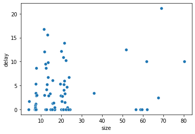
4.2- Delay in shipment
optimal_df = optimal_state_progression.copy(deep = True)
optimal_df['delivery_time'] = optimal_df.groupby(['org', 'dest', 'pickup_time', 'size'])['time'].transform('max')
optimal_df.drop_duplicates(subset = ['org', 'dest', 'pickup_time', 'size', 'delivery_time'], inplace = True)

benchmark_df = benchmark_state_progression.copy(deep = True)
benchmark_df['delivery_time'] = benchmark_df.groupby(['org', 'dest', 'pickup_time', 'size'])['time'].transform('max')
benchmark_df.drop_duplicates(subset = ['org', 'dest', 'pickup_time', 'size', 'delivery_time'], inplace = True)
df = optimal_df[['size', 'pickup_time', 'delivery_time']]
df['delay'] = df['delivery_time'] - df['pickup_time']
##take out everything after the last decision epoch T
df = df[df.pickup_time <= 250]
sns.scatterplot(data = df, x = "size", y = "delay")
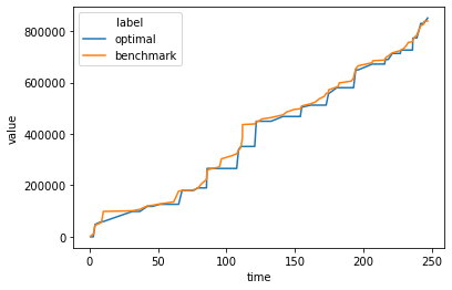
4.3- Cumulative revenue
df1 = pd.DataFrame(data = list(
                     zip(optimal_realized_value,
                         list(optimal_df['time'][1:]),
                         ['optimal' for _ in range(len(optimal_realized_value))]
                        )),
                   columns = ['value', 'time', 'label'])
df1['value'] = df1['value'].cumsum()
df2 = pd.DataFrame(data = list(
                     zip(benchmark_realized_value,
                         list(benchmark_df['time'][1:]),
                         ['benchmark' for _ in range(len(benchmark_realized_value))]
                        )),
                   columns = ['value', 'time', 'label'])
df2['value'] = df2['value'].cumsum()
df = pd.concat([df1[0:250], df2[0:250]], ignore_index = True)
sns.lineplot(data = df, x = "time", y = "value", hue = 'label')
4.4- Error adjusted results
#print('normal error: ', sum(normal_error_trucks))
print('underestimate error: ', sum(underestimate_error_trucks))
underestimate error: 25.0
error_df = normal_error_state_progression.copy(deep = True)
error_df['delivery_time'] = error_df.groupby(['org', 'dest', 'pickup_time', 'size'])['time'].transform('max')
error_df.drop_duplicates(subset = ['org', 'dest', 'pickup_time', 'size', 'delivery_time'], inplace = True)

df = optimal_df[['size', 'pickup_time', 'delivery_time']]
df['delay'] = df['delivery_time'] - df['pickup_time']
##take out everything after the last decision epoch T
df = df[df.pickup_time <= 250]
sns.scatterplot(data = df, x = "size", y = "delay")
df1 = pd.DataFrame(data = list(
                     zip(normal_error_realized_value,
                         list(optimal_df['time'][1:]),
                         ['normal error' for _ in range(len(normal_error_realized_value))]
                        )),
                   columns = ['value', 'time', 'label'])
df1['value'] = df1['value'].cumsum()
df2 = pd.DataFrame(data = list(
                     zip(underestimate_error_realized_value,
                         list(benchmark_df['time'][1:]),
                         ['underestimate' for _ in range(len(benchmark_realized_value))]
                        )),
                   columns = ['value', 'time', 'label'])
df2['value'] = df2['value'].cumsum()
df = pd.concat([df1, df2], ignore_index = True)
sns.lineplot(data = df, x = "time", y = "value", hue = 'label')