Optimal staff level using dynamic job shop scheduling

A company operates bases in the US where vehicles depart from and arrive to. Very broadly, the company provides several types of services. For their operation, they need to staff the bases with technicians and customer representatives. The primary goal is to improve how they staff by aligning it better with the volume of arriving and departing vehicles. With this, they are hoping to reduce under- and over-staffed moments, improve customer service and reduce labor costs.

Simplified overview.

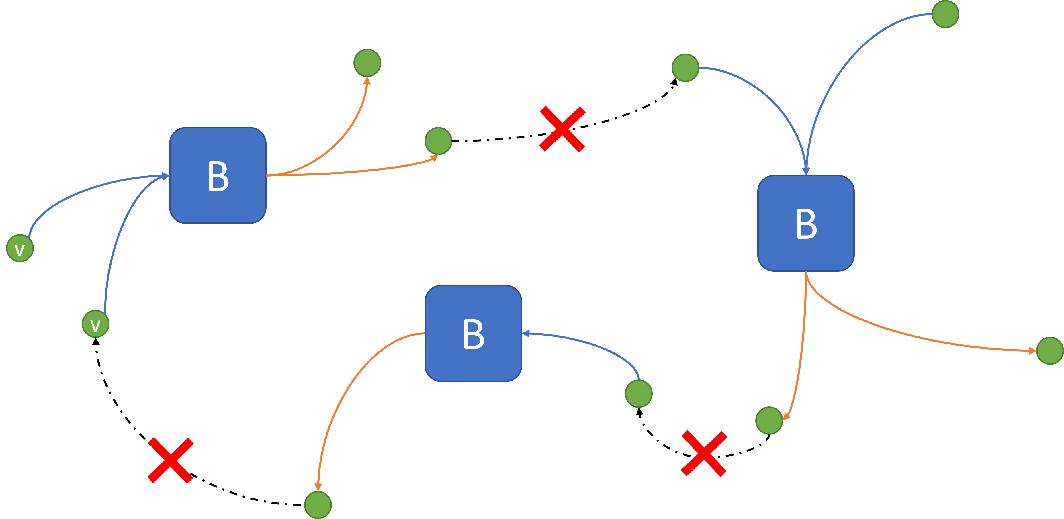
The simplifying overall assumption in the above representation is that the vehicles departing from one base do not arrive to another base from a modeling perspective. This might not hold true in reality but will allow us to solve the optimal staffing level for each base independent of other bases. The assumption will not be limiting as a vehicle departing from one base can still visit other bases, however, their arrival time (or arrival distribution) will be independent of their departure.

The rough solution

The solution framework proposed here will provide the optimal staffing level with respect to the three following business concerns:

• reduce under- and over-staff moments
• improve customer service
• reduce labor costs

This framework consists of a master optimization problem which is modeled within the dynamic programming paradigm and balances staffing level in each shift such that the expected total staff cost over a period of time (e.g., one month worth of shifts) is optimal. The expectation is with respect to the demand level in each shift with three sources of randomness:

• arrival time of vehicles
• service sequence of each vehicle
• serving time for each service type

DP formulation of the master problem

It is assumed that the staff level within each shift are constant and cannot be changed. Therefore, the decision maker can only change staff level when the previous shift is over and before the next shift starts. It is also assumed that once a vehicle arrives at the base, its service request is known and remains the same throughout vehicle’s stay at the base.

State space

Let \((t, t')\) denote start and end time of a shift. Define vector \(V_t = (v_1, \ldots, v_n)^t\) to store the information of vehicles which are present (or have arrived) at a base by the start of shift \(t\). For each vehicle \(v^t_i\in V_t\), its status, remaining service sequence, and its arrival time are recorded, i.e.,

\[v^t_i := \Big(I_{v_i}, \big\{(m_j, p_j)|_{j=1}^J\big\}, \tau^0_{v_i}\Big)\]

where the status variable, \(I_{v_i}\), is \(1\) when the vehicle’s service sequence is started, and \(0\) when the vehicle is idle and waiting for its turn to start service. \(\big\{(m_j, p_j)|_{j=1}^J\big\}\) denotes the vehicle’s random service sequence where \(j=1,\ldots,J\) shows all the services that the base can offer, \(m_j\) is \(1\) if vehicle \(v_i\) has requested service \(j\), and \(0\) otherwise. \(p_j\) is the exponential random time required for service \(j\). The arrival time of a vehicle at the base is also recorded by exponential random variable \(\tau^0_{v_i}\).

In addition to vehicle’s information, the staffing level in each shift is also required to make appropriate decisions for next shift’s optimal staff level. Let \(R_t = (r_1, \ldots, r_J)^t\) denote the vector of staffing level at the start of shift \(t\) where \(r_j\) shows the number of staff level for service type \(j\) for all \(j=1, \ldots, J\).

Therefore, the state variable which summarizes the system’s information at the start of each shift is given by

\[S_t := (V_t, R_t)\]

Action space

At each decision epoch, i.e., after the end of each shift (or before the start), the decision maker can change increase or decrease the staff level for each service type. This action is captured by the following decision variable

\[X^t := \{x^t_j:\, \forall j=1,\ldots,J\},\]

where \(x^t_j\) denotes the increase\decrease in number of staff for service type \(j\) in shift \(t\).

Immediate cost structure

Increasing or decreasing the level of staff for each service type incurs a different cost/reward which is captured by parameter \(C_j\) for \(j=1, \ldots, J\). Therefore, increasing the number of staff for service type \(j\) by \(x^t_j\) at the start of shift \(t\) incurs a cost of \(C_j x^t_j\) while decreasing the staff level by the same number would return a revenue of \(-C_j x^t_j\). This structure will be later referred to by the function \(h(S_{t+1}, S_t, X_t)\).

Optimal equation

The master problem’s objective is made up of two components:

• cost/reward of increasing/decreasing staff level between subsequent shifts
• the revenue produced in each shift as a function of the shift’s staff level

where the first component is defined and given by Section 2.3 and is realized before the start of next shift, the second component is the direct result of staff scheduling within shift \(t\). Let \(W_{t}(S_t)\) show the expected net return of shift \((t, t')\) when the system is in state \(S_t\) at the start of shift \(t\).

\(W_t(S_t)\) will capture three different cost/reward components:

• Revenue for finishing a vehicle’s service sequence realized only when the sequence is finished.
• Penalty for each vehicle’s idle time before its service sequence starts
• Penalty for idle times of each server within shift \((t, t')\)

These components depend on how the vehicles’ service sequences are assigned to available workers. In industrial engineering terminology, this is usually referred to by Job-shop scheduling. The aim of an optimal job-shop schedule is to assign a series of jobs to different workers (machines), typically, to reduce the entire time span of job completion or maximize worker utilization.

Therefore, capturing these cost/reward components motivates solving a job-shop scheduling sub-problem in each shift \((t, t')\). This setup has another advantage which is the optimal determination of the state of system at the end of each shift, i.e., \(S_{t'}\). For more details refer to Section 2.5.

Assuming all cost/reward components of \(W_t(S_t)\) are captured by solving the job-shop scheduling sub-problem, the optimal equation of the master problem is given by

\[\max_{X_t} \, \mathbb{E}\Big[\sum_{t=0}^{T} W_t(S_t) + h(S_{t+1}, S_t, X_t) \Big| S_0\Big]\]

for which the optimal solution is equivalent to the solution of the following Bellman’s equation

\[W_t(S_t) = \max_{X_t} \mathbb{E} \Big[h(S_{t+1}, S_t, X_t) + W_{t+1}(S_{t+1})\Big| S_t\Big]\]

State dynamics

Evolution of the system from \(S_t\) to \(S_{t+1}\) is governed by the function \(f(S_t, X_t, \omega)\) where \(\omega\) is a random element representing the system’s three sources of randomness (see Section 1). Recall that \(S_t\) summarized vehicle and staff level information at the start of shift \(t\). Vehicle information is subject to change while the shift is in progress as new vehicles might arrive at any time during a shift, they will have their own unique service sequence, and the time to finish serving is also random.

Moreover, vehicles which are present by the start of shift \((t, t')\) are also subject to state variable change as they move along their service sequence. Therefore, the system evolves from \(S_t\) at the start of shift to \(S_{t'}\) at the end. This evolution depends on the three identified sources of randomness and also on how the servers were assigned to each job in shift \((t, t')\).

Unlike vehicle information, server information \(R_t\) remains constant while shift \((t, t')\) is in progress. However, this information is subject to change when the shift is over and the decision maker can increase/decrease the number of staff for each service type \(j\) before the start of next shift. Therefore, one can think of function \(f(S_t, X_t, \omega)\) as a two stage function where

\[f(S_t, X_t, \omega):=\left\{\begin{array}{l} S_t \xrightarrow[\text{job-shop scheduling}]{\text{random element } \omega} S_{t'}\\ \\ S_{t'} \longrightarrow S_{t+1}: S_{t+1} = (V_{t+1}, R_{t+1}) = f(S_{t'}) = (V_{t'}, R_{t'} + X_t) \end{array}\right.\]

To model the first stage evolution, random sources of information must be modeled first: (i) The arrival a new vehicle is modeled via a Poisson process where each vehicle’s arrival time is given by an exponential distribution such that \(t^0_{v_i} \sim \exp(\lambda_b)\) where \(\lambda_b\) is the expected time before next arrival for base \(b\) and is evaluated by fitting the data to an exponential distribution. (ii) Each vehicle arrives with a different sequence of services required. This is captured by fitting the data to a cumulative distribution where each vehicle’s new sequence is distributed according to \(p(\{m_j\}|_{j=1}^{J})\sim F({m_j}|_{j=1}^{J})\). (iii) Each service type’s serving time can also be modeled via an exponential (or normal) distribution, where \(p_j\sim\exp(\lambda_j)\) where \(\lambda_j\) is the expected time of finishing service type \(j\).

NOTE that assuming an exponential distribution will allow us to use the memoryless property which comes with its own advantages and disadvantages. For example, if a specific service is not finished by the end of a shift, the memoryless property will allow us to generate a new time to finish serving without tracking how much time was spent on the service in the previous shift. These assumption allow for simulation of these random processes within the dynamic framework. Note that these random processes provide the opportunity to utilize external variables to estimate these distribution parameters. Examples could include weather conditions effects on arrival distribution.

The second factor that affects the evolution of the system from state \(S_t\) at the start of shift to state \(S_{t'}\) at the end of shift, is the result of the job-shop scheduling sub-problem which is explained in more details in the following Section 3.

IP formulation of job-shop scheduling sub-problem

Assume that at the start of each shift, all the servers are free and available and a sequence of remaining jobs are given for optimal scheduling. To ease notation, this draft will skip formulating the job-shop scheduling sub-problem as it is a well-studied problem in the optimization community. The reference section at the end of this proposal includes a number of articles for variations of this problem.

Here, an overview of the objective function, its constraints, and the setup within the master problem’s state evolution will be described. Note that a typical job-shop scheduling problems requires the following information: Number of jobs, the sequence of operations (services) for each job, number of servers for each operation, and processing (serving) time for each service type. All of these information is available at the start of each shift by state vector \(S_t\).

Decision variables

For ease of notation, only a brief description of each decision variable is given here:

• \(u_{i,j,k}\) is 1 if server \(k\) of type \(j\) is selected to carry service type \(j\) of vehicle \(i\)
• \(s_{i,j,k}\) denotes the start time of service type \(j\) of vehicle \(i\) for staff \(k\) of type \(j\)
• \(c_{i,j,k}\) denotes the completion time of service type \(j\) of vehicle \(i\) for staff \(k\) of type \(j\)

• \(y_{i, i', j, k}\) is 1 if service type \(j\) of vehicle \(i\) precedes service type \(j\) of vehicle \(i'\) for staff \(k\) of type \(j\)

• \(c_i\) denotes the completion time of serving vehicle \(i\)

Objective function

The main factor in the objective function of this job-shop scheduling problem is the revenue generated by finishing a job, i.e., completing a vehicle’s service sequence. This is easy to capture by associating a positive dollar value to \((t' - c_i) \times \$\) which encourages the objective function to finish service sooner rather than later ( contributes to improved customer service, revenue generation, and reducing under-staff moments). The second factor is penalizing the vehicle’s idle time before its service sequence starts. This can also be captured by associating a negative dollar value to \((s_{i,j_1,k} - t^0_{v_i})\times \$\) where \(s_{i,j_1,k}\) is the start time of the first service type \(j_1\) in the service sequence of vehicle \(i\) by staff \(k\) and \(t^0_{v_i}\) is the arrival time of vehicle \(i\) which is known from the state variable ( could contribute to improving customer experience, and reducing under-staff moments). The final factor in the objective function is penalizing server idle time which can be captured by associating a negative dollar value to \((s_{i,j,k} - c_{i', j, k})\times \$\) if \(y_{i, i', j, k} = 1\) ( capturing over-staff moments). NOTE that the objective function could be customized to capture different business needs and priorities by tuning the relative weight of these components or adding new components.

Therefore, the objective function of the job-shop scheduling is incentivized to finish service sequence of vehicles, starting service sooner rather than later, and keep a high staff utilization.

Constraints

The job-shop scheduling problem is typically formulated with the following constraints:

• Each service (operation) is given to only one staff
• Each staff is assigned to one job at a time
• Service precedence where start time of a service type for vehicle \(i\) should be after completion of the previous service type according to the vehicle’s service sequence
• The difference between completion time of a service type \(j\) by staff \(k\) and start type of the next service type \(j\) by the same staff \(k\) should be at least the processing time (serving) of service \(j\), i.e., \(p_j\)

These constraints could also be customized to capture different business needs and requirements.

Setup

As the job-shop scheduling problem is framed within the master DP formulation, there are additional setup considerations required to accommodate arrival of new vehicles. At the start of shift, the remaining sequence of services for each vehicle is known. For services that are not finished during the previous shift, a new processing time will be generated. All the staff will be available for job assignment and a regular job-shop scheduling problem can be solved.

As the shift progresses, new vehicles may arrive and update the state vector \(S(t)\). Each time a new vehicle arrives, the job-shop scheduling must be solved again if staff are available. If a new vehicle arrives, and staff is not available, the job-shop scheduling must be solved again as soon as a staff becomes available. To do that, consider these additional constraints

• First come, first serve rule by which service type \(j\) of vehicle \(i\) by staff \(k\) takes precedence over service type \(j\) of vehicle \(i'\) if arrival time of vehicle \(i\) is before vehicle \(i\), i.e., \(t^0_{v_i} < t^0_{v_i'}\)
• Service non-preemption by which once a service starts it cannot be interrupted before its completion even if the shift changes or a new vehicle arrives. To implement this constraint, services that are not finished by arrival of a new vehicle or the end of a shift, are hard coded into decision variables for next solution.

Solution and impact

The sub-problem will not be a huge integer programming problem and should be solvable in matter of seconds by existing solvers. The overall master problem does not have an exact analytical solution but the Bellman’s equation is shown to be greedy-optimal in the long run for a one-step look-ahead policy. At each time, it is assumed that the next shift is the last shift. Then, the dynamic programming framework can be simulated one step into the future and the optimal policy for this one-step look-ahead problem can be obtained. Then, the horizon rolls over one-step into the future with the optimal solution and the process repeats.

Note that the master problem’s objective function has a component to reduce the labor cost by the end of horizon \(T\). The job-shop scheduling sub-problem generates revenue by finishing vehicle’s service sequence while it is incentivized to reduce delay of service and keep staff utilization high. The overall effect of this setup should reduce under-staff moments because job completion contributes positively to the objective. It should be able to reduce over-staff moments because the objective tries to keep utilization high and reduce labor costs. It should also improve customer service since the objective’s aim is to finish as much as it can in one shift and it also penalized the delay of service.

Moreover, the dynamic programming paradigm allow for real-time implementation of this framework. Once the model is trained over a sufficiently long period, it should be able to produce optimal staff level and optimal schedules one period at a time by one-step look-ahead simulation. This has the benefit of reacting to changing circumstances on the ground in an online fashion.

Simulation and testing

The solution methodology for solving this dynamic programming formulation takes advantage of simulation. Therefore, the setup for simulating the optimal solution and comparison with the current practice already exist once the problem is solved one time. Actual arrival times, service times, service sequences and level of staff will be given to the one-step look-ahead simulation framework and the optimal solution for one shift will be produced. The optimal schedule (given by the optimal staff level) can be compared to real practice in terms of service finish time, staff utilization, and vehicle idle times in addition to the cost/revenue generated by both the simulation and the real practice.

References

Hoitomt, Debra J, Peter B Luh, and Krishna R Pattipati. 1993. “A Practical Approach to Job-Shop Scheduling Problems.” IEEE Transactions on Robotics and Automation 9 (1): 1–13.

Nasrollahzadeh, Amir Ali, Amin Khademi, and Maria E Mayorga. 2018. “Real-Time Ambulance Dispatching and Relocation.” Manufacturing & Service Operations Management 20 (3): 467–80.

Özgüven, Cemal, Lale Özbakır, and Yasemin Yavuz. 2010. “Mathematical Models for Job-Shop Scheduling Problems with Routing and Process Plan Flexibility.” Applied Mathematical Modelling 34 (6): 1539–48.

“The Job Shop Problem | OR-Tools | Google Developers.” n.d. Google. Google. https://developers.google.com/optimization/scheduling/job_shop.